Upgrading our Fee Markets to the final form.

In this blog, I explore “Dynamic Pricing For Non-fungible Resource: Designing Multidimensional Blockchain Fee Markets.”

A natural thing to wonder while viewing this tweet is wondering about the waste of resources and compute. A subsequent question is, what makes it possible? Is it because the resources are being priced too cheap? We’ll come to this problem again in a bit.

Blockchains are public ledgers that allow users to submit transactions that modify the shared state. Full nodes with finite computational resources verify these transactions. How does a transaction try to secure a spot in this block? Many blockchains today enable smart contract development. Smart contracts are basically just programs that run on-chain. Users interact with these programs in the form of transactions, and these are executed by full nodes and added to a “block.” Interacting with these programs in the form of transactions requires some fees the network charges, which can be considered compensation for transaction processing.

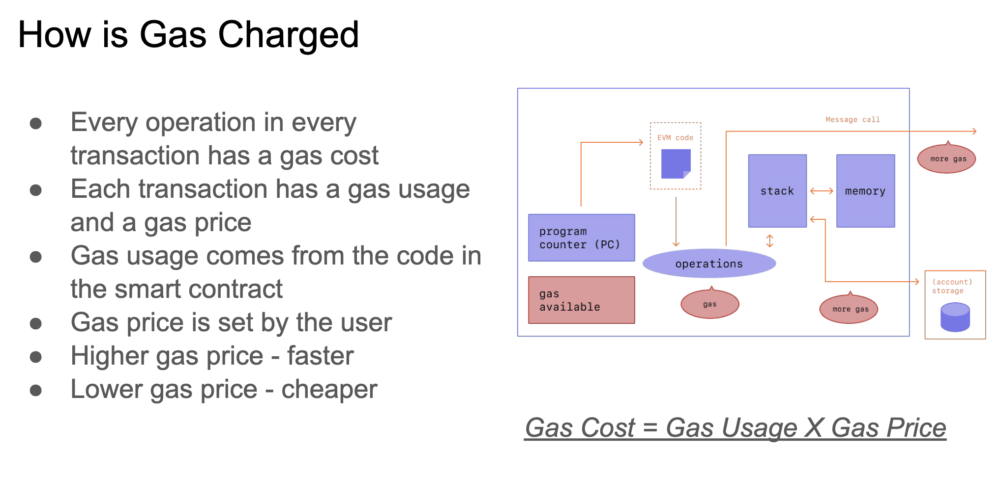
What unit of account do these blockchains charge for this? In the case of EVM (Ethereum virtual machine), this unit of account is gas. Each operation in the EVM requires a hardcoded amount of gas. Earlier, we mentioned that blockchains limit the resources consumed in a unit of time. In this case, the unit of time is done on a per-block basis, and the limit is called the block limit, which enforces a “limit” on the total amount of gas consumed. Since there’s only a fixed supply and the demand for this fluctuates, so does the price of “gas” (as demand-supply theory would dictate).

Blockchains face the fundamental challenge of balancing limited computational resources with fluctuating user demands. Transactions compete for block inclusion, consuming network bandwidth, storage, and computation. However, blockchains like Ethereum rely on a fungible unit like gas to price these resources. This makes it hard to reflect each underlying resource's actual marginal cost and scarcity.

In the paper “Broken Metre: Attacking Resource Metering in EVM,” Perez et al. show a way of a new DoS (Denial of Service) attack on ethereum exploiting this one-dimensional “metering” of resources and propose the Resource Exhaustion attack. The essence of the attack is exploiting the fact that there were EVM instructions for which the gas fees were too low compared to the resources they consumed. This also led to an EIP-2929, which increased the gas requirement for these opcodes for some of the EVM instructions mentioned in the paper. There were also similar attacks like this on the SUICIDE opcode in 2016.

Let’s do a thought experiment: Imagine you live in an apartment building where all utilities - electricity, water, heating, etc. - are bundled into a single bill that all residents split evenly. This means you pay the same monthly amount as your neighbor even if you barely use electricity or water, and they crank up the heat and AC all day. In this scenario, you have no incentive to conserve scarce resources others depend on. You end up overconsuming cheap resources like electricity while underutilizing resources like heat that you don't personally value as much (or need).

The same issues crop up when blockchains price computation, storage, and bandwidth using one fungible token. You may want to store a large file on-chain while someone else is running complex smart contracts. But you pay gas proportionally to the total resources used, not based on your specific demands. This leads to mispricing and misallocation of scarce non-fungible resources. Computation may be overutilized, while storage is underutilized. There is no way for the market to express the actual marginal cost and demand for each resource.

Ideally, we want the price for each resource to reflect its real-time scarcity so the blockchain charges higher fees when bandwidth is constrained versus when computation is plentiful. This would enable more efficient allocation and usage based on actual supply and demand dynamics.

In their paper "Dynamic Pricing for Non-Fungible Resources," Diamandis et al. propose a systematic way to define and update dynamic prices for blockchain resources like computation, bandwidth, and storage. This is done by formulating an optimization problem from the network designer's perspective to maximize transaction utility minus resource loss. The problem decomposes into two parts - minimizing network loss and maximizing transaction producer welfare - joined by resource prices.

Note: This article will be pretty convex optimization heavy, and the reader is suggested to have some familiarity. However, I’ll try to motivate what the equations mean and signify at every step.

---

Exploration of Fee Markets

Rollups and Data markets

Rollups are a scaling technique that separates transaction execution from data availability. Transactions are executed off-chain in a rollup, with only transaction data posted to the base layer. The roll-up occasionally submits proof of valid state to the base layer. This naturally creates two separate fee markets - one for including transaction data on the base layer and one for execution in the rollup.

Some "lazy" blockchains exclusively are optimized for data availability, leaving the execution to rollups that have also popped up. This also creates separate markets for data inclusion and execution.

Ethereum has proposed allowing notable "blob" transactions containing arbitrary rollup data in EIP-2242 and then expanded upon in EIP-4484. Blobs can be priced separately from base layer gas, creating a two-dimensional fee market. Decoupling execution from data availability unlocks scalability and thus no longer constrains the base chain.

In a proto-danksharding (EIP-4484) implementation, all validators and users still have to directly validate the availability of the full data.

The main feature introduced by proto-danksharding is new transaction type, which we call a blob-carrying transaction. A blob-carrying transaction is like a regular transaction, except it also carries an extra piece of data called a blob. Blobs are extremely large (~125 kB), and can be much cheaper than similar amounts of calldata. However, blob data is not accessible to EVM execution; the EVM can only view a commitment to the blob. - From Proto-Danksharding FAQ

Independent fee markets for data and execution enable more precise price discovery based on actual supply and demand. Overuse of one resource won't congest the other. Adding a blob/data market alongside base layer gas avoids competition between rollups and base layer transactions. Rollup data has a dedicated channel. Overall, separate fee markets for data availability and execution are a natural fit for rollup architectures. This prevents congestion across purposes and improves efficiency through targeted pricing. The multidimensional fee model proposed in the paper formalizes how to implement such markets.

Proto-dank sharding introduces a two-dimensional EIP-1559 fee market with separate floating gas prices and limits for regular gas and blobs. There are two resources: gas and blobs. Each has a target per block (15M gas, eight blobs), a max per block (30M gas, 16 blobs), and a variable basefee. The blob fee is charged in gas but adjusts based on blob usage to target eight blobs per block on average. Block builders face a more challenging optimization problem balancing gas and blob limits and maximizing revenue. Heuristics can get close to optimal. The exponential EIP-1559 adjustment mechanism for blobs fixes issues with the current EIP-1559 formula, making adjustments depend only on total usage. The fake_exponential function approximates the exponential adjustment while being simple and efficient to compute. In summary, proto-dank sharding creates a two-dimensional fee market to utilize block space better and avoid worst-case usage scenarios. The new exponential blob fee adjustment provides better targeting.

Parallelization

There are two main approaches to enabling parallel execution in blockchains:

1. Minimal VM changes and the responsibility is shifted to full nodes to identify parallelization opportunities.

2. Using access lists - Transactions specify which accounts they access so that Non-conflicting transactions can be executed in parallel. This is used in Solana Sealevel to unlock parallel processing for thousands of transactions.

The issue with the access list approach is that contention for popular accounts limits parallelization gains. Many transactions want to access the same accounts (NFT mints, popular protocols, or presales), forcing sequential execution.

We also saw Easy Parallelizability being discussed for Ethereum, and this was discussed as a way to speed up the EVM in a blog by flashbots. In the end, we will see a formalization of fee markets for threaded VM resource pricing.

Exploration by Ethereum and Solana

In ethereum, a multidimensional fee market was proposed by Vitalik in the form of Multidimensional EIP1559.

Ethereum has resources with different bursts (short-term) and sustained (long-term) capacity limits. For example, the EVM can handle occasional slow blocks but not sustained ones. The current gas model doesn't handle these burst vs. sustained differences well. It makes worst-case and average-case ratios similar, leading to inefficient gas costs, but the resources used in these cases are vastly different. For example, on average, transaction data plus call data consumes ~3% of the gas in a block. Hence, a worst-case block contains ~67x (including the 2x slack from EIP 1559) more data than an average-case block. The post proposes a multidimensional EIP 1559 - separate EIP 1559 controllers for each resource. Base fees for each resource are adjusted separately based on usage. This allows much higher slack parameters as the entire burst/sustained gap is represented. Limits would rarely be hit except in edge cases. Resources could include EVM execution, call data, witness data, and storage. The benefits noted from this were lower fees from more efficient pricing, better DoS protection, and reduced need for dynamic basefee algorithms. We will not cover a thorough analysis of EIP 1559 and transaction fee mechanism in this blog and refer the reader to Transaction Fee Mechanism Design for the Ethereum Blockchain: An Economic Analysis of EIP-1559 and Transaction Fee Mechanism Design by Tim Roughgarden et al. (We will cover these works in a later blog). One thing to note about EIP-1559 is that although it is close to the problem that this paper considers, it makes the fee estimation problem easier in a way that disincentivizes manipulation and collusion. This paper aims to price resources dynamically to achieve set objectives.

Multidimensional Fee markets are also being considered in a different form. Anatoly Yakovenko proposed it for Solana in “Consider increasing fees for writable accounts.” The issue proposes increasing fees exponentially for unused writable accounts to disincentivize bots flooding the network with invalid transactions based on stale state. The fee design is meant to help build congestion control, capture fees, punish misbehaving senders, and refund well-behaved senders. An alternate proposal suggested increasing fees for used accounts and rebating a portion of the program, giving developers more control while still limiting contention.

---

Defining the Problem

Transactions A transaction in ethereum is defined as any action taken by an externally owned account (i.e., not a smart contract). Suppose A sends B 1 eth. This must be debited from A’s account and credited into B. A transaction changes the state of the EVM.

The data (arbitrary in nature) is sent over the p2p (peer-to-peer) network to be added to the chain. They are first broadcasted and collected by nodes in the mempool. The mempools act as a staging/holding area for pending transactions waiting to be included in the block. Transactions in the mempool are prioritized by various factors, primarily the gas price offered. This is why gas immediately goes up during high volume transaction times because users keep spamming transactions with higher gas fees, so their transaction gets included and is prioritized. A miner/validator gets to choose which transactions from the mempool go into a block. Miners may also outsource this to “block builders.”

Nodes Nodes execute and validate transactions to maintain the latest state. Most blockchains try to have minimum computational requirements for these nodes in a blockchain. They have finite resources, so blockchains limit total resources per unit of time to prevent overload. If transactions are included in a blockchain faster than nodes can execute them, these nodes won’t be able to reconstruct the latest state and, therefore, assert validity. This is also called Resource Exhaustion Attack.

Resource Targets and Limits One way to avoid Resource Exhaustion would be to enforce a fixed upper bound of resources/combination of resources in a unit amount of time (or blocks). Another way would be to ensure miners do not constantly include high-resource transactions to blocks and better manage resource distribution/loading. This would suggest that we should have a “Resource Target” - a minimum target for consumption of resources every block to avoid waste of resources and a “Resource Limit” - so we make sure nodes catch up after a while.

Resources

Most blockchains have several “meterable” resources (as in measurable, and we use this to quantify their usage as well). We will label these resources $i = 1, …, m.$

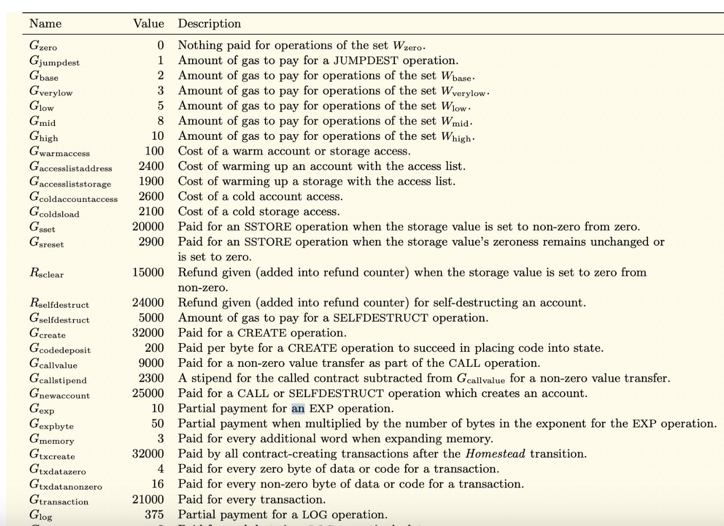
In Ethereum's EVM, the fee unit is gas. Each operation consumes a hardcoded gas amount. As seen below, they all consume resources. We will henceforth only consider resource consumption rather than these granular opcodes (although you could use them if you wanted to).

For a given transaction $j = 1,….n$, we will let $a_j \in \mathbb{R}^m_+$ be the vector of resources that transaction $j$ consumes. In particular, the $i$th entry of this vector, $(a_j)_i$, denotes the amount of resource $i$ that transaction $j$ uses. Basically

If we have three resources that we are trying to measure, let’s say storage, computation, and bandwidth. For some transaction $x$ we could write the vector as $[storage, computation, bandwidth]$. In more concrete terms, taking numbers here $[10, 20,30]$ would be the different resources transaction $x$ consumes. These quantities don't need to be non-negative (E.g., some resources may not consume storage, so that they would be 0).

Okay, another question to ask is, can we consider a combination of resources? What if computation alone doesn’t have much meaning to be considered, and you want to consider computation and bandwidth both? Or what if using computation or storage alone is okay, but using them both is costly? In this case, formally, if you have two resources $R_1$ and $R_2$ you can create a combined resource $R_1R_2$ which can be metered separately. So your vector could look like

$x = [ R_1, R_2, R_1R_2]$

Now that we have representation for resources, we will talk about resources we want to utilize. As we spoke earlier, we want a “resource target,” i.e., we would like to have a sustained amount of resources always being used in the blockchain (ideally). In the case of ethereum, there is a resource target for gas, which is 15M gas per block. Now, since we want to expand it to multiple resources, we will represent it by a vector $b^*$ $\in \mathbb{R}$ with the exact representation as in the resource case, the ith entry denotes the desired target of resource i in a block. The resource utilization of a particular block is a linear function of transactions included in a block written as a Boolean vector $x \in \{0,1\}^n$, which is again a vector.

To understand this as a simple example, let’s say we have five transactions being considered, and the 1st, 2nd, 4th, and 5th are being included in the block. The boolean vector looks like

$x = [1, 1, 0, 1, 1]^T$

Since we have multiple transactions and each transaction consumes its resources, we will represent this as a matrix $A\in \mathbb{R}^{m*n}$ whose jth column is the vector of resources $a_j$ consumed by the transaction $j$. What do we mean? Continuing our example, we have five transactions and three resources each (as mentioned earlier, computation, storage, and bandwidth). So, an example matrix looks like

$A = \begin{bmatrix}12 & 32 & 34 & 43 & 54 \\1 & 2 & 3 & 4 & 5\\10 & 20 & 30 & 40 & 50\end{bmatrix}$

If we want to write this block's total quantity of consumed resources, we will write it as $y = Ax$.

In our example

$y = Ax$

$y = \begin{bmatrix}12 & 32 & 34 & 43 & 54 \\ 1 & 2 & 3 & 4 & 5 \\ 10 & 20 & 30 & 40 & 50\end{bmatrix} * \begin{bmatrix}1 \\ 1 \\ 0 \\ 1 \\ 1 \end{bmatrix}$

$y = [141, 12, 120]$

where the $ith$ entry is the $ith$ resource consumed by all transactions included in the block (for reference $[storage, computation, bandwidth]$).

Now, if we want to measure the deviation of resources from our target, we would subtract our total resources used and the resource target we had. So, we want to measure the deviation between the Resource total given by $Ax$ and the Resource Target $b^*$ Formally

$Ax-b^*$,

is another vector whose $ith$ element gives the deviation for the $ith$ resource. (positive or negative, positive would mean more resources used, negative would mean less resources used compared to resource target).

Finally, we also mentioned we will have a Resource limit. We don’t want any valid block to use resources greater than the resource limit we set. We will represent it by $b$.

Formally, $Ax \leq b$. In the case of ethereum, gas (single resource) has a limit of 30 million gas per block.

There we have it. We have represented how to measure the various resources, calculate deviation, and represent the resource limit.

Network Fees

Now that we have formulated the things we want. We will now express the fees. As we mentioned earlier, fees are charged by the network for transactions (i.e., for operations that are done in a transaction). We want to ensure its set so that the usage is close to the resource target, not the limit. If transaction $j$ with resource vector $a_j$ is included in a block, a fee $p^Ta_j = \sum_ip_i(a_j)\_i$ is paid to the network. A natural thing to assume now is that as the resource keeps getting scarce, any additional amount required is costlier than it would have been otherwise (supply-demand law).

Note: In Ethereum, the network fee is implemented by burning some amount of gas (post EIP 1559).

Resource Mispricing Given A (the block of transactions) and b (the resource limit), it is not very obvious how to set fees $p$ to ensure the network performs well.

One Example we should note is the transaction spam attack, which is called the EXTCODESIZE opcode repeatedly, an attack that happened in 2016. This exploited mispriced resources since EXTCODESIZE was too cheap and caused the network to slow down a lot. When you attempt a full node today, you can see a dramatic slowdown and processing from block 2283416 to 2463000. This immediately led to a subsequent EIP-150, which fixed the issue with the hardfork. This incident makes us realize the importance of resource pricing appropriately and not neglecting this problem since it can directly affect the performance of the underlying chain.

A simple Idea

Lets now think of a simple rule for $p$:

• if $Ax =b^*$, there is no update since we have reached the resource target.

• If $(Ax)_i >g b^*_i$, increase $p_i$ to reflect this.

• If $(Ax)_i < g b^*_i$, decrease $p_i$ since we have not reached the basic resource target.

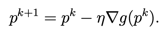
How do you update p in the next block, though? This equation can be given by

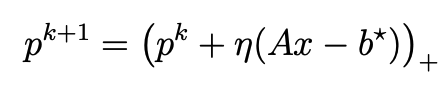
where,

• $p^k$ is the vector of prices for each resource at iteration $k$

• $η$ is the learning rate - this controls how big of an update step we take. If we make this too big, then the jump in the fees from one block to the next will be too high, thus making the network unusable. If we make it too small, the fees might be too low to reflect the demand that the resources are under right now and, hence, might lead to spam.

• $Ax$ is the observed resource utilization from the transactions included in the latest block

• $b^*$is the target resource utilization

In words, it is:

New prices = Current prices - Learning rate * (Observed usage - Target usage)

(A slight aside for interested readers: This equation is an example of the gradient descent update rule for iteratively adjusting the weights of the network, but instead of $Ax-b^*$, you would have the loss.)

This type of iterative price update rule based on supply and demand motions (a different motivation in other spaces) appears in many contexts. Still, it is especially prevalent in machine learning for optimization and multi-agent learning. The goal is always to gradually steer behavior toward an optimal point, just like tuning the prices in a blockchain fee market.

Resource Allocation Problem

The ultimate goal of this system is to maximize the utility of the underlying blockchain. Since we are not omniscient, we do not know what the inclusion of a transaction in a block means to a user or miner (i.e., the utility) or what they want to add to a block. So, most of our optimization/design is around the desire to modify the fees so that resource usage is always near the resource target.

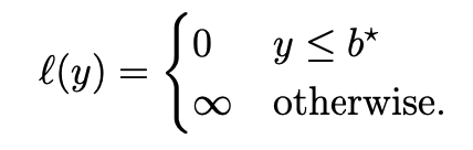
Loss Function - We define a loss function to somehow measure the “dissatisfaction” or the unhappiness of the network designer. We assume only that $\\ell$ is convex and lower semicontinuous. Assuming a function is convex makes it more efficient to optimize and also makes it so that the function has one optimal (global minima in the case of a convex function) value (that we are trying to find). Semicontinuous means that the optimization process is stable and that some minimum exists.

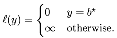
We observe two equations below. The first design of the loss function says we are only okay if the resource utilization $Ax$ or, in other words, $y$ is always equal to the resource target $b^*$. The second one basically encodes the notion that we are happy if $y$ is less than $b^*$ but unhappy otherwise.

While there are other losses we can consider, one important one is calculating the per-resource utilization.

Each loss function in some form ultimately expresses what the network designer wants to optimize for and capture tradeoffs as well. These choices result in a separate update rule (like the one we saw earlier) for the network fees $p$.

Resource Constraints $S$ represents the set of valid transaction bundles users and miners can create and include in a block. This set can encode various constraints:

1. Hard limits on resource consumption like Ax ≤ b

2. Contention for popular accounts or contracts

3. Interdependencies between transactions

So, S captures all the limitations and complexities around which transactions can be bundled together in a block. A reader who has followed us till now might be confused about why $S$ exists in the same world as $x$ since we mentioned that $x$ also denotes the transactions included in the block. The best way to think about this is S defines the finite, discrete set of transaction bundles that could end up in x based on real-world constraints. S represents "This is what is actually possible," while x represents "This is what miners chose." This is also why we have the constraint $x \in S$.

Convex hull of Resource Constraints The convex hull conv(S) contains all convex combinations of points in S. This allows the network designer to "average" transactions over multiple blocks. Specifically, components of x can vary continuously between 0 and 1, interpreted as the probability or fraction of including a transaction over many blocks. Taking the convex hull conv(S) relaxes the binary constraints, allowing "partial" transactions. This relaxation allows the designer to reason about long-term resource utilization rather than allocation in a single block. This does not mean users or miners will create partial transactions. It's a convenience for the designer. Users/miners can only include transactions fully or not at all. The convex hull allows the designer to model allocation in an idealized way. This will allow the problem to decompose nicely into two coupled subproblems: one solved on-chain and one off-chain with integral solutions.

Transaction utility We define transaction utilities in the form of $q \in \mathbb{R}^n$. $q_j$ represents the joint “utility of miners and users” for including transaction $j$ in a block of $n$ transactions. This is an opaque quantity and very hard to know. The actual values of $q$ don't need to be known. Only users/miners try to maximize utility.

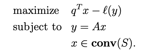
The problem

Where,

• $q^Tx - \ell(y)$ represents maximizing total transaction utility

• The constraint $y = Ax$ enforces that the resource utilization y must equal the resources consumed by the chosen transactions Ax.

• The constraint $x \in conv(S)$ requires the transaction bundle x to be an element of the convex hull of the feasible set S. This allows "partial" transactions.

The interpretation is that this is the "ideal but unrealistic" problem the network designer would solve. The paper shows that this decomposes into two problems: on-chain and implicitly by users and miners. The combination is called transaction producers. This combination exists because it’s inevitable that a user-miner colludes. This possibility was also mentioned in the paper “Transaction Fee Mechanism Design” by Roughgarden et al.

The Dual function

Okay, we defined a problem we couldn’t solve and now need to convert it into a form, so we will.

When dealing with a complex optimization problem, the concept of duality is a powerful tool. The dual problem is a natural counterpart to your original, or "primal," optimization problem. The dual problem is always the opposite of the primal. If the primal is minimization, the dual problem is maximization and vice versa. The dual is appealing because, more often than not, original problems in convex optimization seem to be very difficult but become very solvable in the dual form. What also makes the dual so compelling is that it provides a lower bound for the solution of the primal problem. This is invaluable because it gives you a benchmark for how good your solutions can be. They offer you alternative perspectives for understanding your problem, simplify complex equations, and can even lead to more efficient algorithms.

In the primal problem above, we were optimizing a constrained optimization problem.

We first pull in the $x \in conv(S)$ into our resource constraint problem to obtain

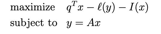
where I is an indicator function which is 0 if $x \in conv(S)$ and $+\infty$ otherwise. (As we said earlier, we want our x only to be within what’s possible. It’s meaningless to us otherwise).

We add the constraints to the objective function to form the Lagrangian using dual variables (Lagrange multipliers). The dual for this problem is defined by

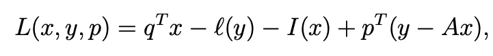
where the constraint gets added to the original problem and $p^T(y-Ax)$ represents a penalty.

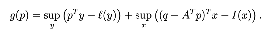
Rearranging, we finally find the dual function,

Where,

• $p$ is the Lagrangian dual variable (also called the price) that relaxes the equality constraint $y = Ax$

We aim to maximize the Lagrangian L(x,y,p) over x and y.

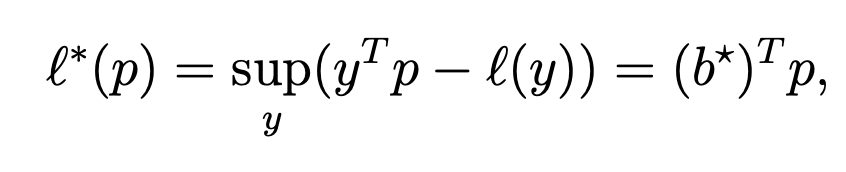
The first time in the above equation is the Fenchel conjugate of the resource constraint problem evaluated at $p$. We will write it as $\ell^*(p)$.

The Fenchel conjugate is a key concept in convex analysis and duality theory. Given a function$f(x)$, the Fenchel conjugate $f^*(y)$ is defined as:

$f^*(y) = sup_x ( y^T x - f(x) )$

Where "sup" refers to the supremum or least upper bound.

Intuitively,$f^*(y)$ represents the maximum value that can be obtained by matching the function $f(x)$ with a linear function $y^T x$. It captures the best possible alignment between $f(x)$ and its linear approximation.

Some key properties of the Fenchel conjugate:

• $f^*(y)$ is a convex function, even if $f(x)$ is nonconvex. This makes it very useful in convex optimization.

• The conjugate "flips" maximization and minimization. Maximizing $f^*(y)$ is equivalent to minimizing $f(x)$.

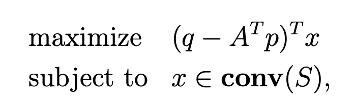
The second term defines the transaction producers' problem, and it optimizes the following problem

Where,

• $q$ is the transaction utility vector. $q_j$ is the utility of including transaction $j$ in the block.

• $A$ is the resource matrix, where column $j$ is the resource vector $a_j$ consumed by transaction $j$.

• $p$ is the resource price vector set by the network.

• $x$ is a binary vector indicating which transactions are included in the block.

So $(q - A^Tp)^Tx$ is the total utility to transaction producers of the transactions included in $x$ (the utility $q_j$ of each transaction $j$, minus the fee paid to the network $p^Ta_j$ for that transaction's resource usage).

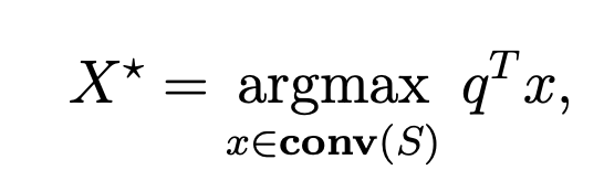
This is maximized subject to the constraint $x ∈ conv(S)$, which means $x$ is in the convex hull of the set of possible/valid transaction bundles $S$.

So, in other words, the second term is finding the set of transactions x that maximizes the transaction producers' total utility, subject to x being a valid transaction bundle. We will write the second term regarding p as $f(p)$. This is a convex function.

We write the dual function as

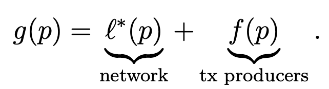
Since both the parts are convex, $g(p)$ is also a convex function.

The dual problem

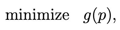
The dual problem is to minimize $g$ as a function of the fees $p$. By optimizing over p, We align incentives across the network and transaction producers to achieve an optimal system-wide outcome.

Under certain regularity conditions, the functions $\ell^*$ and $f$ are differentiable, and their gradients can be characterized as:

$∇l^(p) = y^*$

$∇f(p) = -Ax^*$

where $$$y^*$maximizes$p^Ty - l(y)$and$x$maximizes$(q - A^Tp)^Tx$over$conv(S).$$

Therefore, the gradient of the overall dual function is:

It states that the optimal prices $p^*$ equalize the resource usage target $y^*$ with the realized usage $Ax^*$ induced by the transaction producers at those prices.

In essence, the optimal fees align the incentives of the network (to minimize its loss l(y)) and the transaction producers (to maximize their utility) by properly internalizing the costs. The optimal fee that should be charged is the exact marginal cost the network faces.

Now, we provide conditions under which the optimal resource prices/fees p* will be non-zero.

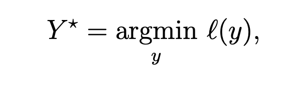
We define two disjoint sets, where $X^*$ is the optimal set of transactions included when resource fees are 0 and $Y^*$ is the set that minimizes the loss.

The condition we then have is

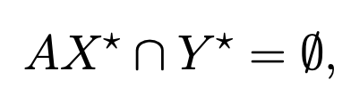
In other words, if the resource usage $AX^*$ induced by the zero-fee demand $X^$ does not overlap at all with the optimal usage $Y^*$ that minimizes network loss, then the optimal prices $p^*$ must be non-zero. Intuitively, this means that if the users/miners want to include transactions at zero price that incur some network loss, then the network must charge non-zero fees $$$p^$to align incentives. Fees guide behavior away from zero-fee demand$AX^$*toward the optimal usage*$Y^*$$.

This motivates the need for multidimensional pricing. With separate prices for each resource, over-utilization of one resource can be discouraged by increasing its fee, while under-utilization of another can be encouraged by decreasing its fee.

There are some properties we can derive from dual problem about the prices $p$:

• First, the optimal price p* must be non-negative.

• Second, it defines a condition on the loss function called superlinearity, which implies that the domain where the dual function g(p) is finite is precisely the nonnegative orthant. This means the optimal prices are restricted to be non-negative. Superlinear losses prevent unbounded subsidies.

• Third, it characterizes the maximum prices beyond which transactions that consume resources will not be included by users/miners. This helps bound the range of reasonable fee values.

Overall, the properties guide setting resource prices and characterizing their behavior. The nonnegativity constraints reflect the increasing costs of higher network usage. And the maximum prices bound subsidies and prevent exclusion of all resource-using transactions. The takeaway is that despite its generality, the structure of the network loss function $l(y)$ and dual function $g(p)$ enable valuable insights into the optimal pricing of blockchain resources.

The Solution

We can iteratively converge to the optimal prices. In a less constrained environment, L-BGFS could work.

But since on-chain environments are compute-constrained (like that on ethereum), the paper suggests a modified version of gradient descent that is easy to compute and does not require storage beyond the fees.

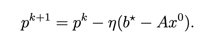
In gradient descent, we have

Where $\eta$ is the learning rate and if g is differentiable, we use the derivate to update the prices. This works well when g(p) is differentiable. The update direction is guaranteed to reduce g(p).

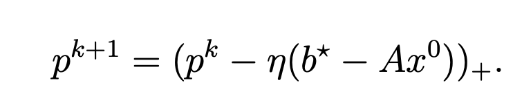
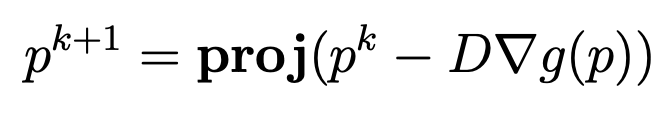
To ensure p stays in the domain of g, the paper suggests using projected gradient descent:

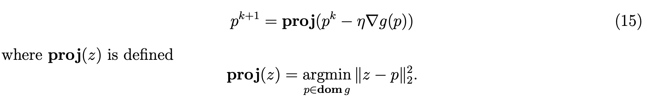
where proj(z) projects $z$ onto the domain of $g$.

Now, evaluating the function $g$ at point $p^k$ is not always possible. We saw earlier if $g$ is differentiable, it only depends on the solutions to the two terms.

Let $y^*$ be a maximizer of the $sup_y(p_k^T y - l(y))$, which is easy to compute in practice, and we replace $x^*$ with the observed solution $x^0$. Since this $x$ is boolean, we compute resource usage $Ax^0$ after observing the included transactions.

We can then use an updated form.

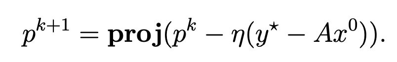
We see that this equation increases the network fee for a resource being overutilized and decreases the network fee for a resource being underutilized. As you would expect, this pricing mechanism is designed to disincentivize future users and miners from including transactions that consume currently overutilized resources in future blocks. This is not the only algorithm that works for this.

The paper gives a few examples of loss functions and the update rules we get from them.

Consider our earliest loss function,

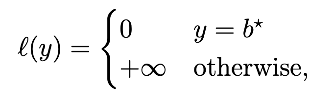
The conjugate function we get is

where the optimal value of $y$ is $b^*$. The update rule is,

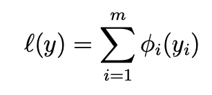
Consider another loss function: linearly separable losses

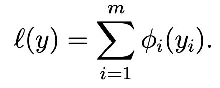
The loss comes out to be

While the papers use the gradient descent rule for this, other modifications can be considered, like adding momentum and adaptive steps.

Extensions of the Fee Market

Parallel Transaction Execution

Consider L parallel execution threads, each with its resources plus shared resources. The transaction run on thread $k$ is denoted by $x_k \in {0,1}^n$.

The allocation problem is given by:

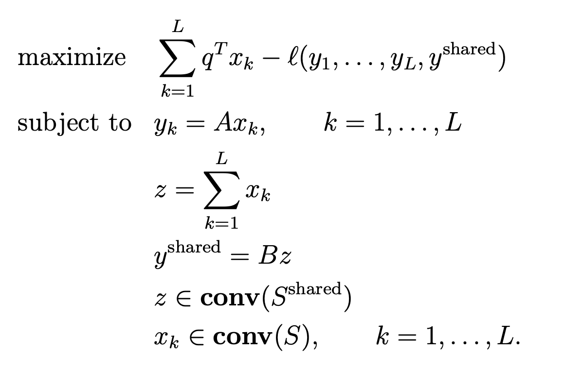
where,

• Transactions $x_k$ are allocated to thread $k$.

• Resource usage is $y_k = Ax_k$ per thread, $y_{shared}$ = $B_z$for shared resources, where $z = Σ_k x_k.$

• Resource allocation problem is to maximize utility minus loss.

• This can be solved using the same duality approach by combining all resources into one vector.

• It enables pricing threads and shared resources separately.

Different Price Update Speeds

• The premise is that some resources can sustain burst capacities for much shorter periods of time compared to other resources. Therefore, Some resources may need faster price adjustments than others.

• Introduce per-resource learning rates $η_i$ to update resource prices $p_i$ for resource $i$ faster when needed.

• Update rule becomes

where, $D = diag(η_1,...,η_m)$.

We can also define this problem on a per-contract utilization basis instead of per resource.

Conclusion

We explored multi-dimensional fee markets in this blog. In future blogs, I will explore transaction fee mechanism design.